Poisson Goodness of Fit Test Tutorial

When to use this tool

The Poisson Goodness of Fit Test is a statistical tool used to check whether a set of count-based data follows a Poisson distribution. The Poisson distribution is often used to model events that happen randomly and independently over a fixed period of time or space, such as:

• The number of customer calls received by a help desk per hour
• The number of machine breakdowns in a factory per week
• The number of medical errors in a hospital per month

This test helps determine if the observed data matches what we would expect under a Poisson model. If the test shows a good fit, it means the event happens randomly at a constant average rate. If the test does not fit well, it suggests that other factors might be influencing the event, such as patterns, clustering, or external influences that make the event non-random.

Using EngineRoom

Click to Download Data File

A hospital's safety committee is investigating the frequency of workplace accidents in its clinical laboratory. Over the past year, they recorded the number of minor lab-related accidents (e.g., chemical spills, needle pricks, equipment malfunctions) occurring each week. The committee wants to determine if the number of accidents follows a Poisson distribution, which is often used for modeling rare event occurrences over fixed intervals.

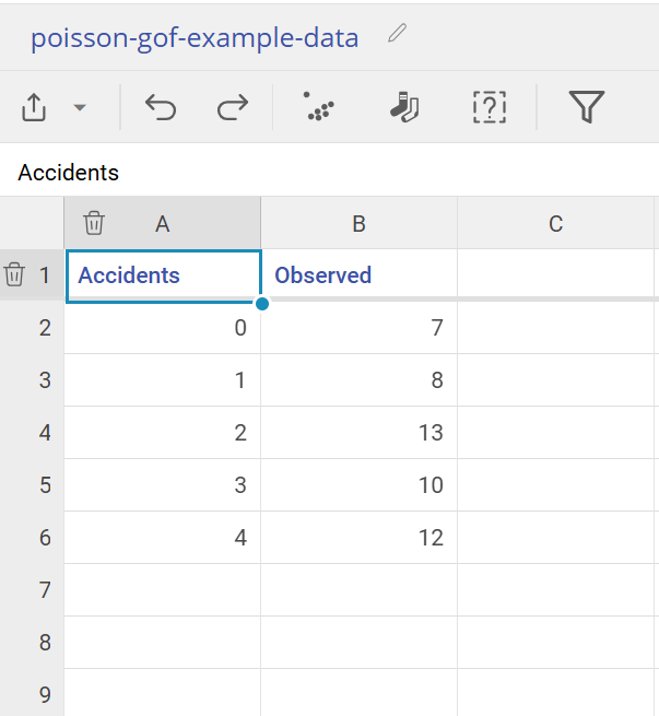
The data contains "Accidents", which is the count of accidents that occur within a given week, and "Observed" which is the number of weeks that the number of accidents occured.

Select the Poisson Goodness of Fit test from the Parametric menu under Analyze.

Example:

Note: This example has the Guided Mode disabled, so it combines some steps in one dialog box. You can enable or disable Guided Mode from the User menu on the top right of the EngineRoom workspace.

Steps:

• Select the Analyze menu > Parametric > Poisson Goodness of Fit
• Click Continue to move past the Example Data screen.

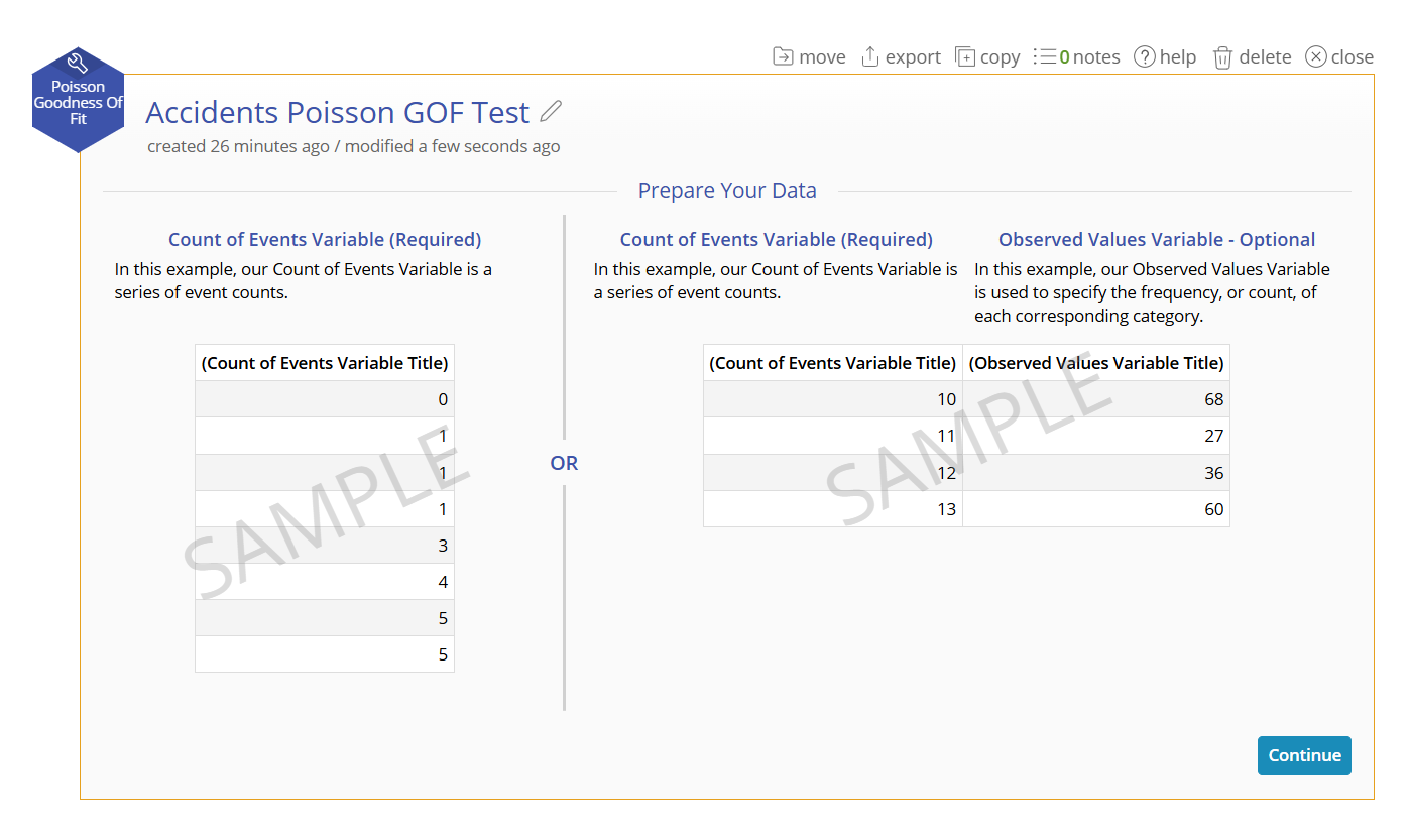
• Drag the Accidents variable onto the Count of Events Variable drop zone on the study:

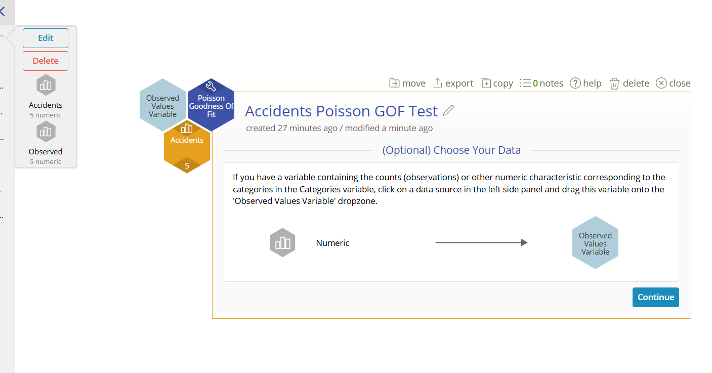
• Drag the Observed variable onto the Observed Values Variable drop zone on the study:

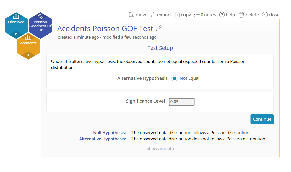
• On the Test Setup screen, the alternative hypothesis is always the not-equal to case (see the null and alternative hypotheses spelled out at the bottom of the study screen). However, the significance level can still be changed. In this case, we will leave it at the default of 0.05.

• Click Continue to see the Poisson Goodness of Fit test output:

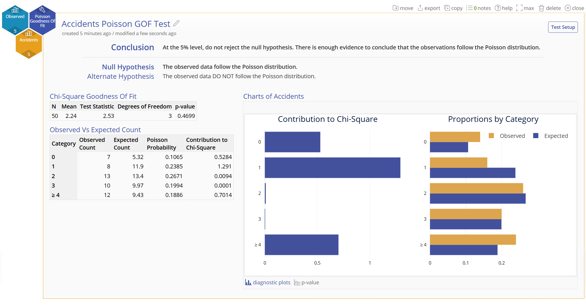
The conclusion statement states the results of the test in plain English, followed by the null and alternative hypothesis statements.

The numeric output on the left shows the Test table showing the total sample size, mean, test statistic for Chi-Square Goodness of Fit, degrees of freedom and p-value. In these results, the p-value is 0.4699, which is greater than the chosen alpha value of 0.05, so you fail to rejectthe null hypothesis and conclude that observed values are not significantly different from the Poisson Distribution.

The Observed vs Expected Count table shows the actual number of observations in each category in the sample and the number of observations that you would expect to occur if the test proportions were true, along with the Poisson Probabiliy and the Contribution to Chi Squared.

The graphical output on the right shows the diagnostic plots. The Chart on the left is a graphical representation of the Contribution to Chi-Square, while the graph on the right shows the observed and expected counts.

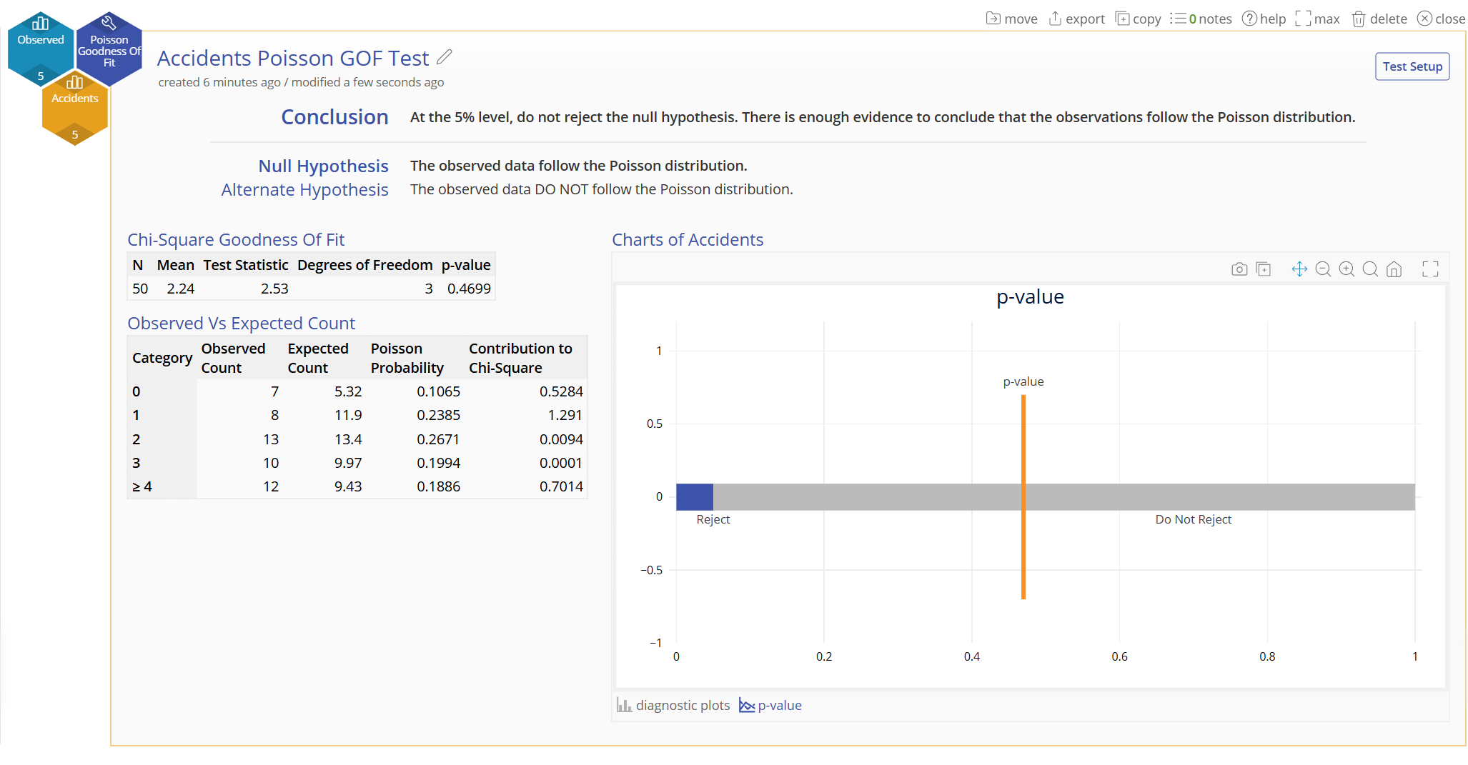
The p-value chart can be seen by clicking the link next to the diagnostic plots link - it shows the p-value falls within the blue rejection region for the test:

A Note on Sample Size

In general goodness of fit tests are ideal when the total sample size is between 75 and 150. Too few or too many samples the test can be overly sensitive. To mitigate this, in a goodness of fit test, the minimum cell size should be 5. The test is highly sensitive when cell sizes are 0 or 1.

Poisson distributions will always have at least a tail to the right. As the mean gets above 7-8, a Poisson distribution will also have a tail to the left. The implication is that as the tail(s) drift off, there will be small expected and observed values. Unlike in a classic Chi-squared table with expected counts that are non-zero, a Poisson distribution will have values that the expected value will be 0 while there could be an observed count with those values. The Chi-Sq calculation blows up with an expected count of 0, so cells must be collapsed.

In order to account manage this, on the tail(s) observed and expected counts will be merged such that expected count will be at least 2 (consistent with Minitab’s approach). The problem with merging to 5 is that too much emphasis is placed in the tail area of the distribution, especially as the sample size is small.

In running simulations with data that was Poisson distributed, n=2 seems to be fairly robust in managing the risk in placing too much emphasis in the tail area. As data becomes more or less dispersed relative to a Poisson distribution, n=2 still manages to capture issues with the data.

Other Notes:

• If you have raw data - that is, data listing each category as it occurs, you can use this test to evaluate whether the data categories have equal proportions (a uniform distribution.)

Poisson Goodness of Fit Test Video Tutorial

Coming Soon